The Bayer Process (the process of extracting alumina from bauxite) is an energy-intensive technology, consuming large amounts of fuel and energy. This Alumina or aluminium oxide (Al2O3) is then used to produce Aluminium at a ratio of 2:1. However, did you know that around 75% of aluminium ever produced is still in use in some form today? It is one of the most recyclable materials available and can be recycled over and over, using only 5% of the energy required for producing the original metal, thus somewhat off-setting the high amounts of energy required for its initial production.
The flow of fluids within the alumina process can be simulated with FluidFlow. Friction loss of Newtonian fluids such as water, steam and sodium hydroxide solution are calculated using the normal Darcy equation/Moody diagram method. (The compressible flow calculation is particularly sophisticated taking into account the expansion of the gas and associated temperature and physical property changes. Sonic conditions are also handled. For predicting all physical properties of water FluidFlow uses the IFC-97 formulations developed by the International Association for the Properties of Water and Steam).
Pure Bayer liquors: green/pregnant liquor (or spent liquor) are also Newtonian fluids but with varying physical properties depending on their make-up, for instance, total alkali content etc. The viscosity, density, vapour pressure and thermal properties would have to be determined separately, but once this is complete, the values can be quickly defined in the FluidFlow fluids database for use in a model.
These fluids can also be used as the carrier fluids for suspensions in the Bayer process, say when the hydrates are precipitated. These would be regarded as settling slurries and simulated as described above, using an appropriate correlation such as Wilson-Addie-Sellgren-Clift.
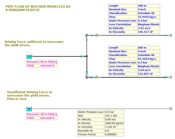
At the very end of the Bayer process we are dealing with a non-Newtonian/non-settling slurry, the “red mud”. Figure 1 shows this type of fluid simulated as a Bingham plastic. In Figure 1, the pipes are of different diameter. Consequently, the shear rate is different and therefore the calculated apparent viscosity is different for each pipe. This example also illustrates the concept of yield stress. In the lower pipe, the driving force is insufficient to overcome the yield stress of the fluid and so, there is no flow in the line.
The properties of this red mud were entered into the fluids database where its viscosity correlation was defined as a Bingham plastic.
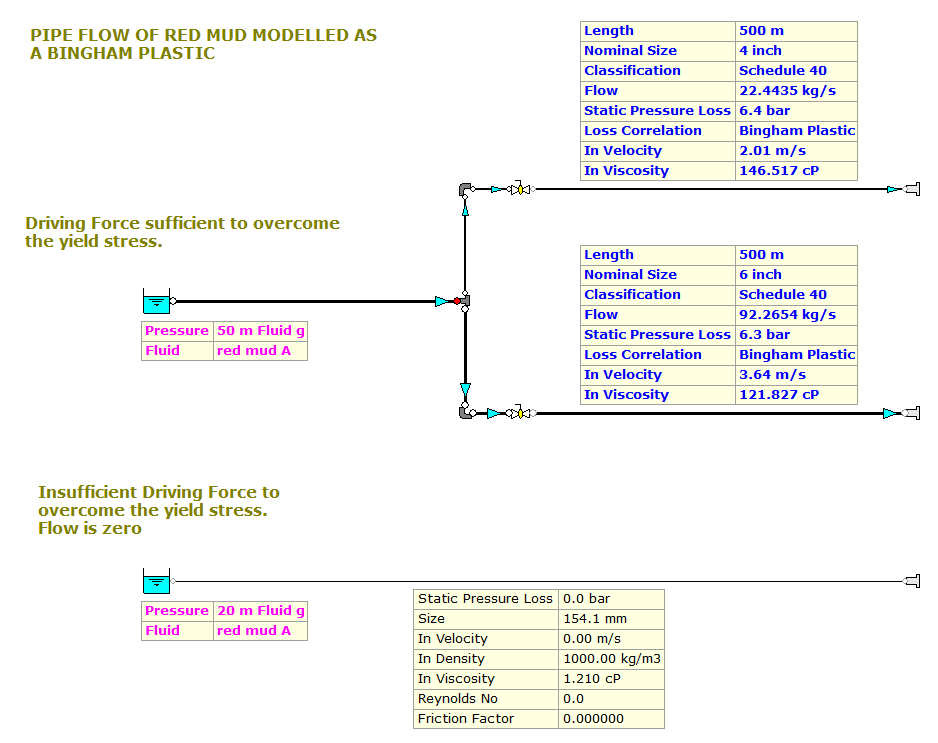
Figure 1: Red Mud – Bingham Plastic.
References: